Big O Notation Explained

Why is Big O Notation Used?

When you got different algorithms to solve the same problem, you need to compare those to each other to pick the best (meaning fastest) for your program. Looking at each algorithm’s (pseudo-) code will give you an insight into how they work and what data structures they rely on. However, that doesn’t tell you how long you have to wait until the algorithm finishes and how the algorithm scales when you increase input data size. To figure that out, you could go through every line of code and determine how often it is executed depending on the input size as we did in the article on insertion sort. This gives us a function \(T(n)\) telling us how often the lines of code are executed depending on the input size \(n\) in the worst-case.

This \(T(n)\) includes all constant factors and all \(n\)s. For a simple polynomial function, such as \(T(n) = an+bn^2+d\) coming from the insertion sort example, figuring out the highest power is easy. However, \(T(n)\) can become quite complex and doesn’t require many code lines. Because of this smart mathematicians came up with a notation that tells us the upper bound of a function and its growth behavior towards infinity. This notation is called the Big O notation.

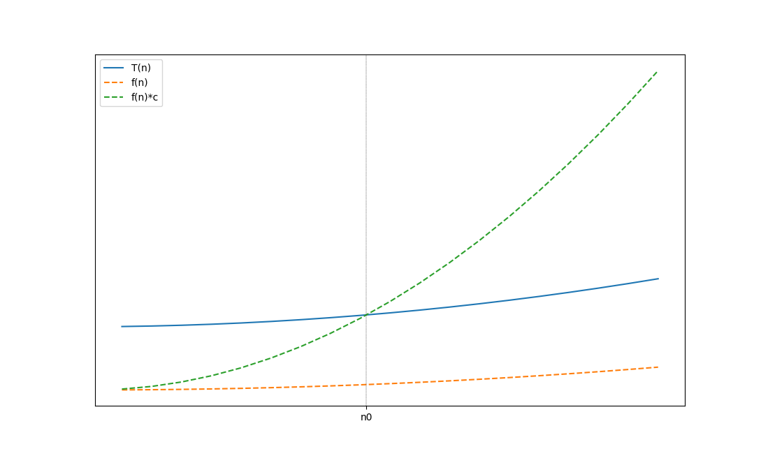
For our function \(T(n)\) we can say \(T(n) \in O(f(n))\) if and only if \(T(n)\) is eventually (meaning after a certain \(n \geq n_0\)) bounded by \(f(n)\) multiplied with a constant \(c\). This tells us, no matter how big \(n\) gets \(T(n)\) will never be bigger than \(f(n)\cdot c\). Looking back at the insertion sort example we can state

if and only if we can find a \(n_0\) and a \(c\) such that \(\forall n\geq n_0: f(n)\cdot c \geq T(n)\). This mathematic notation might be a bit abstract, but let us look at the following figure.

There are three different functions. The solid plotted function our \(T(n)\) the lower dashed lined is \(f(n)\) and the most rapidly growing is \(f(n)\cdot c\). And at \(n_0\) \(T(n)\) is the bounded by \(f(n)\cdot c\) towards infinity and therefore we can say \(T(n) \in O(f(n))\).

Prove Worst Case Time Complexity Example

To mathematically prove that \(T(n) \in O(f(n))\) we have to pick an \(n_0\) and a \(c\) (that are independent from from \(n\)) and show that \(\forall n\geq n_0: f(n)\cdot c \geq T(n)\). Taking the result from the insertion sort \(T(n) = an+bn^+d\) we can show that \(T(n) \in O(n^2)\). First let us pick a \(c\) that is equal to the absolute sum of all coefficients of \(T(n)\):

Then we choose \(n_0=1\). Now we have to show that the following inequality is satisfied:

This means we have to transform/extend \(T(n) = an+bn^2+d\) such that it looks like the inequality above. Firstly, we can state that the function that takes the absolute values of all coefficients is always equal or greater than \(T(n)\):

We can further say that if all powers of \(n\) are equal that the inequality is still satisfied:

Now we can transform the term on the left such that we only have one \(n^2\):

and this is already the inequality from above, and it is true for all \(n_0 \geq n\) \(\blacksquare\)

Worst Case Time Complexity

In computer science, it is established that the big O notation describes the worst-case run time and therefore provides a save upper bound for the algorithm run time. Coming back to our initial problem of comparing different algorithms to each other. We can quickly check and compare their run times for large inputs and their scaling behavior when we have the big O notation of all algorithms. For example, algorithm \(A\) has a worst-case run time of \(T_A(n) \in O(n)\) and an algorithm \(T_B(n) \in O(1)\) it is immediately apparent that \(B\) will always be faster than \(A\) for a sufficiently large input size \(n\) and because of this \(B\) should be chosen instead of \(A\).

Constant Time Complexity O(1)

Algorithms those worst-case run time is in \(O(1)\) have a constant time complexity, meaning, no matter how large the input gets, they will always take the same amount of time to finish their computation. An example for constant time complexity are Python dictionaries:

1
2
3
4
5
6
7

avengers = {
	'Natasha Romanoff': 'Black Widow',
	'Tony Stark':  'Iron Man',
	'Peter Parker': 'Spider Man',
	'Clint Barton': 'Hawkeye',
	'Bruce Banner': 'The Hulk'
}

The avengers dictionary above allows us to access the hero name for a given real name with time complexity of \(O(1)\) because Python dictionaries are based on a so-called hash function that takes the key as an input and the output points to a container containing the value.

Linear Time Complexity O(n)

We could also create a list of tuples for getting the hero name and search for a real name which would look like this:

1
2
3
4
5
6
7
8
9
10
11
12
13
14

avengers = [
	('Natasha Romanoff', 'Black Widow'),
	('Tony Stark',  'Iron Man'),
	('Peter Parker', 'Spider Man'),
	('Clint Barton', 'Hawkeye'),
	('Bruce Banner', 'The Hulk')
]

real_name = "Bruce Banner"

for key, value in avengers.items():
	if key == real_name:
		print(value)
		break

However, we would have to check every entry in that list to find the hero name for a given real name in the worst-case. This puts us into linear time complexity \(O(n)\).

Polynomial Time Complexity O(nˣ)

As we have already proven above, the insertion sort algorithm is in \(O(n^2)\). Sometimes the power of \(n\) can be spotted by how many nested loops an algorithm has. For example, the naive matrix multiplication algorithm is in \(O(n^3)\) because there are three nested loops, and each loop has to be completely iterated from the start to the end:

1
2
3
4
5
6
7
8
9
10
11
12
13
14
15
16
17
18
19
20
21
22

# 3x3 matrix
A = [[8, 2, 1],
     [3 ,7, 9],
     [5 ,4, 6]]

# 3x3 matrix
B = [[5,8,1],
     [6,7,3],
     [4,5,9]]

# 3x3 * 3x3 = 3x3
C = [[0,0,0],
     [0,0,0],
     [0,0,0]]

# iterate through rows of A
for i in range(len(A)):
    # iterate through columns of B
    for j in range(len(B[0])):
        # iterate through rows of B
        for k in range(len(B)):
            C[i][j] += A[i][k] * B[k][j]

Logarithmic Time Complexity O(log(n)) or O(n·log(n))

Between linear and linear and constant time complexity are algorithms having a logarithmic time complexity. Those algorithms usually involve binary trees and recursion. Examples are merge sort and binary search.

Exponential Time Complexity O(xⁿ)

Even though algorithms with exponential worst-case time complexity are very dangerous to work with as they can easily explode the run time of your programs, those algorithms are prevalent. For example, the traveling salesman problem is an algorithm in \(O(x^n)\) because to find the optimal route to visit each station while traveling the shortest distance requires you to try out every possible route, which is exponentially many. However, there are a lot of algorithms that find near-optimal solutions while having a non \(O(x^n)\) worst-case time complexity.

Comparing different big Os

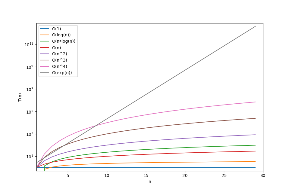
The chart below shows us how different big O grow depending on their input. The x-axis of this plot is actually in logarithmic scaling otherwise it would not have been possible to see the other graphs because \(O(exp(n))\) grows so fast that it reaches a value higher than \(10^11\) with only 30 input elements.

Choosing or designing a clever algorithm that can solve your problem in a small amount of time, meaning and scales nicely for a large input, is one of the critical competencies of a computer scientist as algorithms with bad scaling behavior are often unusable.